🎯 Calibration (files)

City Scanner In-Situ Calibration and Deployment: A Manual

By An Wang (an_wang@mit.edu) – Senseable City Lab, MIT

info

A PDF version is available here.

1 Getting to know City Scanner

1.1 Background

Mobile environment monitoring is a fast-developing method capable of providing high spatial resolution information on air quality, noise, heat, and meteorology. It has been attracting prominent attention from the scientific community and the public for a wide range of applications, including tracing emission sources, evaluating ambient air pollution distribution, and estimating personal exposures. The City Scanner project initiated by the Senseable City Lab at MIT is a pioneer in mobile environment monitoring. It aims at developing a sensing platform to enable large-scale environmental sensing tasks using existing urban fleets as sensing nodes. We envision the platform to be adopted as a novel type of city infrastructure to enable big data collection and evidence-based environmental/climate policymaking.

In general, City Scanner adopts a low-cost, modular design with internet-of-things (IoT) capabilities. Environmental sensing can be expensive and high maintenance in the traditional approach. United States Environmental Protection Agency (US EPA) defines that any air sensor for single or multiple pollutants costing less than $2500 is considered low-cost. Sensors used on the City Scanner are generally less than $500 and are tested with good accuracy and precision. City Scanner implements a modular design for its on-board sensors to lower unit costs even more. Users can easily keep redundant sensing modules to a minimum and adapt the platform in different urban environment deployments. City Scanner is also IoT-enabled, where individual sensing units are mounted on top of urban fleets for data collection and stream data to the cloud for storage, manipulation, and analysis via a cellular network. Jointly, these designs have made City Scanner a leading mobile sensing platform to empower environmental scientific research, support evidence-based environmental and climate decision-making, and encourage citizen engagement and awareness in environmental justice topics.

1.2 Sensing modules on a City Scanner

We illustrate City Scanner version ‘Flatburn’ that is being used for multiple data collection campaigns in global cities in Figure 1. Each City Scanner has two major modules: the core and sensor modules. The core module houses the motherboard, the data communication and local storage system, and the battery and thermal performance management system. The sensor module, GPS and solar panel are connected to and managed by the core module. The core module design detailsre presented in the hardware and firmware open-source manual. Here, we focus on the sensor module that includes all environmental sensors. Figure 1 demonstrates the anatomy of a baseline sensor module configuration. It contains one optical particle counter, two gas sensors, a temperature and humidity sensor, and a noise sensor.

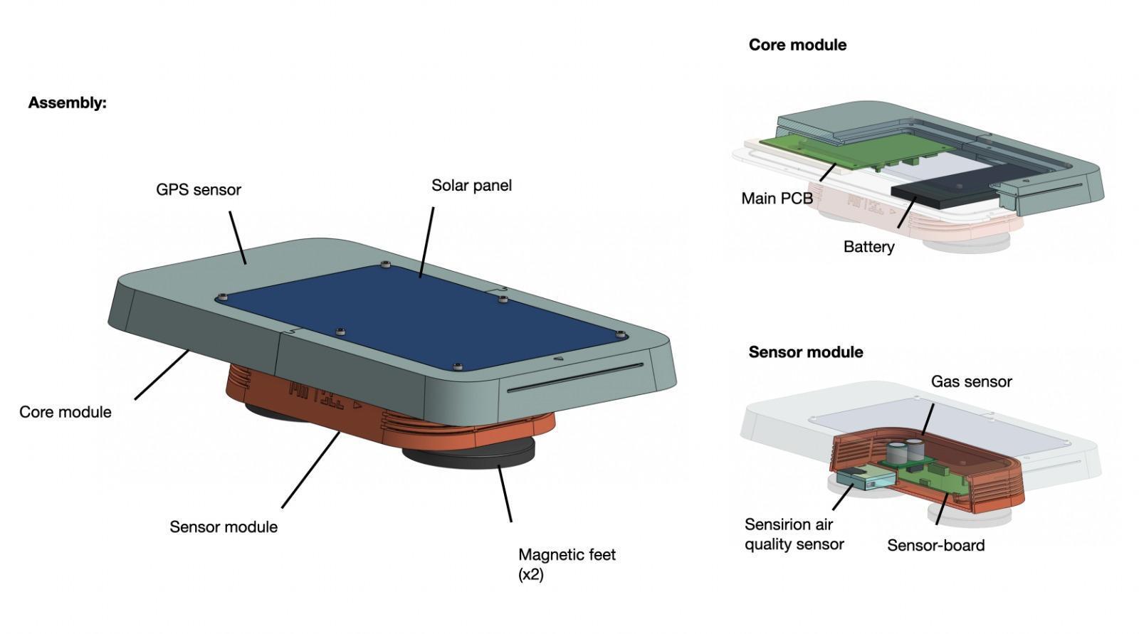
Figure 1. Flatburn basic configuration

We list the environmental sensors that are currently being used in Table 1. Sensirion SPS30 optical particle counter (OPC) is a low-cost sensor for measuring ambient particulate matter (PM). A laser beam is emitted through the air flow being drawn in so that by counting the pulses of light scattered by particles in the air flow, OPC can count the number of particles. Based on the intensity of scatter light, it is also able to measure particle size. Sensirion OPC has been adopted in academic and citizen science projects, whose performance and durability have been proven among other competitors in the market. Two gas sensors can be hosted in the sensor module at the same time.

Currently, we are using Alphasense’s electrochemical gas sensors for CO, NO2, and SO2. The surface material on an electrochemical gas sensor reacts with the target gaseous pollutant, which results in an electric current that passes from the working to the reference electrode. The current is measured and is proportionate to the target pollutant’s concentration. The sensor board can also be equipped with low-cost noise, temperature, and humidity sensors for measurements. But this document mainly explained how air quality sensors are calibrated.

Table 1. Environmental sensor specifications

Sensor	Sensing object	Unit cost	Substitution
Sensirion SPS30 Optical Particle Counter	Particulate matter count and estimated mass concentration	$50	With a thermal camera
Alphasense CO-A4	Carbon monoxide	$50	With other gas sensors
Alphasense NO2-A4	Nitrogen dioxide	$50	With other gas sensors
Alphasense SO2-A4	Sulfur dioxide	$50	With other gas sensors
MIC MEMS Analog	Noise	$50	N/A
BME280	Temperature, humidity	$0.88	N/A

2 Low-cost sensor calibration basics

2.1 The importance of calibration

Low-cost sensors suffer from constant data quality and stability issues. For example, the abovementioned OPC cannot discern particulate matter from water droplets, thus, does not function well in high-humidity environments. Moreover, OPC-observed PM mass concentration is estimated based on particle shape and density assumptions, varying drastically from place to place and season to season. Electrochemical gas sensors are known for their cross-sensitivity, which is a common phenomenon where the electrochemical surface material reacts with gases other than the target one. Therefore, sensor collocation and calibration are of utmost importance to ensure accurate results before field deployment. Collocation is the process of deploying sensors side-by-side with reference monitors and calibration involves adjusting raw sensor readings using collocation data and mathematical methods. We summarized seven issues that affect low-cost sensor performance from low-cost sensor calibration literature within the last five years: intersensor variability, intra-sensor variability, drift, aging, response time, cross-sensitivity, and sensitivity to environmental factors.

Inter-sensor variability refers to the variability in measurements using multiple identical sensors under the same testing environment. The calibration for inter-sensor variability is crucial for low-cost sensors as it is the foundation of large-scale sensor deployment and data transferability. Intra-sensor variability describes the variability in consecutive measurements a given sensor makes under the same testing environment. Drift is the gradual change in sensor response over time. Aging refers to the continuous deterioration of sensor performance over time. Unlike reference sensors, low-cost sensors are prone to drifting and have a much shorter lifetime. Thus, they require routine sensor calibration and replacement. Response time reflects the lag before sensors reach stable readings in the test environment. The difference between response time and temporal signal change scale is critical for time-resolved sampling. Cross-sensitivity, an issue exclusive to gas sensors, denotes a sensor’s false response to gases other than the target gas. Finally, sensitivity to environmental factors, including temperature, humidity, wind, barometric pressure, and particle composition, is ubiquitous in both low-cost and reference sensors. These environmental factors are commonly identified as the main explanatory variables in low-cost sensor calibration models.

2.2 How do people calibrate sensors

The United States Environmental Protection Agency (EPA) is a federal agency that regulates and manages environmental protection matters. They also provide references, guidelines, and regulations considered “the gold standard” for air quality monitoring, primarily in the US and many other countries. In order to facilitate the use of low-cost sensors for non-regulatory purposes, EPA has initiated multiple projects and gathered opinions from various stakeholders. In 2021, EPA published air sensor performance target reports for Ozone and PM2.5 low-cost sensors, which provides consistent testing protocols, metrics, and target values to evaluate the performance of low-cost sensors for non-regulatory applications. Previously, only a few studies followed regulated sensor calibration protocols, whereas most studies developed their own project-specific protocols.

It hinders the inter-project comparison of low-cost sensors. Therefore, City Scanner’s calibration and collocation protocols are mainly developed in conformity with the two reports published by US EPA. In general, there are three phases of low-cost sensor calibration. The first phase is collocation, which indicates a process of deploying low-cost sensors next to reference-grade monitors. Reference monitors are a category of air sensors whose manufacturers, data quality, and durability are certified by government agencies, specifically, EPA in the US. They are considered the gold standard for air pollution monitoring in many regions across the globe. The second phase is calibration, which includes adjusting raw low-cost sensor readings using statistical methods with reference monitor data as the target variable. The last phase is evaluation, where the calibrated results are tested against external reference monitor data (data not used in calibration training) with statistical measures, such as Pearson correlation coefficient and mean absolute percentage error. The three phases are detailed in Section 3.

3 Calibrating a City Scanner

3.1 In-situ collocation setup

US EPA provides two standardized performance test protocols. The base testing involves evaluating sensors in an outdoor environment, and the enhanced testing refers to the evaluation in a controlled lab environment. Enhanced testing is recommended if a laboratory chamber is available but not mandatory. Hence, we will focus on the base testing protocols in the City Scanner context.

City Scanners are recommended to be collocated and calibrated in an environment that is as similar to the deployment environment as possible. That is to say, City Scanners should be calibrated locally at a reference air quality station if it is available and ideally in the same season as the deployment. Considering sensor aging and drifting, if a deployment is more than six months in length, it is highly suggested to have collocation before and after the deployment. Usually, City Scanners are collocated at a reference station for at least two weeks for a single deployment. This would generate over 300 paired hourly readings, which is sufficient to fit a simple multivariate linear regression, but not enough to account for potential nonlinearity between low-cost sensor response and meteorological factors using machine learning algorithms. It is suggested to have a one-month consecutive collocation if time and space allow or require higher temporal resolution reference monitor data (finer than hourly).

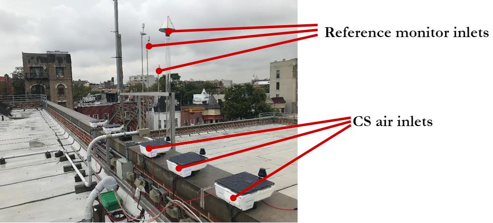
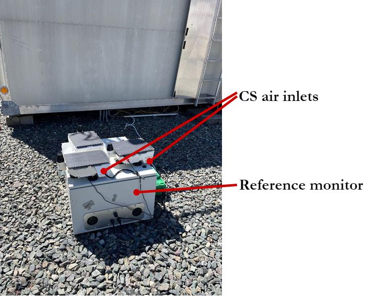
Figure 2 illustrates two previous collocation and calibration campaigns in New York City (NYC) and Boston. The setup in NYC is more desirable. As we can see, five City Scanners are placed next to each other, facing the same direction with a secure connection to a power source. All are very close to the reference monitors’ air inlet. This is important to ensure consistent and continuous monitoring. The reference station is located on the rooftop of a primary school. City Scanners are elevated from the roof, and set securely on a flat platform with no obstruction around them. This ensures free air flow from all directions and minimizes the effects of wake dust. The setup in Boston is not ideal but can still yield valid results. The City Scanners are placed close to the ground instead of the reference monitors’ inlet on the roof of the container in the back, as the power socket is located on the ground. Moreover, our City Scanners are placed quite close to the container that hosts various reference monitors, which induces the risk of not capturing pollutant plumes from certain directions.

(a)

(b)

Figure 2. City Scanner collocation setup in (a) NYC (b) Boston

3.2 Data processing and digest

Collected data can be downloaded directly from the SD card located in the core module. Locally downloaded data are not cleaned and do not have field names attached, which need to be done manually in this case. Figure 4 presents a sample of locally downloaded raw data. Raw data are separated into multiple files for a single deployment. There are three steps before one can use it for calibration or analysis, including combining, filtering, and renaming. First, we need to combine the data files from the same City Scanner in the same campaign. Second, the records marked with ‘0’ in the first column are invalid and should be filtered out. Lastly, the first column needs to be discarded so that all field names can be attached to each column. There are, in total, 46 fields as listed in Table 2. We have provided a simple python script to automate this process.

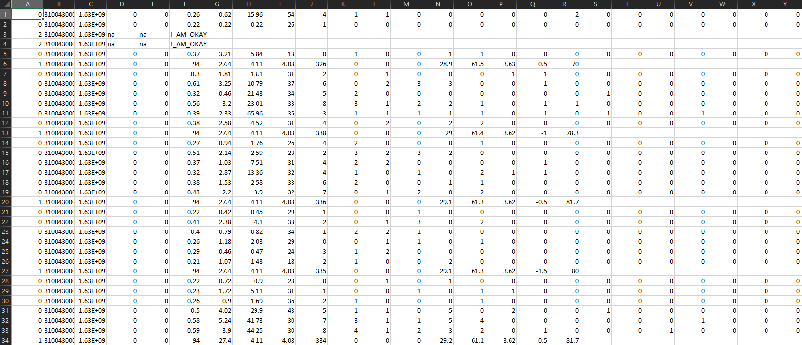
Figure 4. Locally downloaded City Scanner raw data from the previous City Scanner prototype

Table 2. City Scanner data file fields and definitions

Field name	Definition
deviceID	-
timestamp	Time stamp in epoch time
latitude	-
longitude	-
PM1	PM1 mass concentration in ug/m3
PM25	PM2.5 mass concentration in ug/m3
PM10	PM10 mass concentration in ug/m3
flowrate	OPC flowrate at air inlet
countglitch	Possible OPC count errors
laser_status	OPC laser status
temperature_opc	OPC temperature in Celsius
humidity_opc	OPC humidity in percentage
data_is_valid	If OPC data is valid
temperature	Ambient temperature in Celsius
humidity	Ambient humidity in percentage
gas_op1_w	Gas sensor 1 working electrode millivoltage (This is the measurement proportionate to gas 1 concentration)
gas_op1_r	Gas sensor 1 reference electrode millivoltage
gas_op2_w	Gas sensor 2 working electrode millivoltage (This is the measurement proportionate to gas 2 concentration)
gas_op2_r	Gas sensor 2 reference electrode millivoltage
noise	Noise level in dB

Cleaned City Scanner data requires calibration against the reference monitor readings, using meteorological factors as explanatory variables. Previously, we used meteorological factors from a central weather station for all City Scanners circulating in a city, and the calibration performance was satisfactory. Here, we mainly consider four factors that have effects on sensor performance based on a previous City Scanner study, namely, temperature, humidity, air pressure, and dew point. A conceptual calibration function is presented as follows, which can be fitted with multivariate linear regression, but preferably an algorithm that can interpret nonlinearity, such as random forest or gradient boosting trees. It is worth noting that we need to log-transform the reference and City Scanner observations (pollutant concentration) to comply with the normal distribution assumption if needed.

𝑙𝑜𝑔 (𝑟𝑒𝑓 𝑜𝑏𝑠𝑒𝑟𝑣𝑎𝑡𝑖𝑜𝑛) = 𝑓(𝑙𝑜𝑔 (𝐶𝑆 𝑜𝑏𝑠𝑒𝑟𝑣𝑎𝑡𝑖𝑜𝑛) ,𝑡𝑒𝑚𝑝, ℎ𝑢𝑚𝑑, 𝑝𝑟𝑒𝑠, 𝑑𝑒𝑤𝑝)

We have provided some sample codes to demonstrate the calibration process. The sample codes take in synchronized reference air quality observations, City Scanner raw readings, temperature, humidity, air pressure and dew point values that are aggregated to 1 min, 5 min, 10 min, 30 min, or 60 min intervals, which are common temporal resolution one can get from local weather station and reference air quality monitors. Then, log-transformed City Scanner raw readings and meteorological factors (in total,five predictors as in the previous equation) are passed to a variety of calibration algorithms to train the best calibration model for each City Scanner unit. The choice of the best calibration model is made by comparing the performance metrics in Section 3.3.

3.3 Performance metrics and quality assurance

Table 3 lists a series of performance metrics for base testing. It is compiled assuming multivariate linear regression as the calibration algorithm. In reality, meteorological factors have complex interactions with each other and with low-cost sensor performance. It is recommended that other than linear regression, random forest calibration should be tested, which is a simple machine learning model that can account for nonlinearity. As a rule of thumb, at least 500 data points are needed to develop a robust random forest model.

Table 3. Performance metrics for base testing

Test type: Base testing

Metric	Description
Precision	Variation around the mean of a set of measurements reported concurrently by three or more sensors of the same type collocated under the same sampling conditions. Precision is measured here using the standard deviation (SD) and coefficient of variation (CV).
Bias	The systematic (non-random) or persistent disagreement between the concentrations reported by the sensor and reference instruments. Bias is determined here using the linear regression slope and intercept.
Linearity (Important)	A measure of the extent to which the measurements reported by a sensor can explain the concentrations reported by the reference instrument. Linearity is determined using the coefficient of determination (Pearson correlation). As a rule of thumb, Pearson correlation should be over 0.9 after calibration.
Error (Important)	A measure of the disagreement between the pollutant concentrations reported by the sensor and the reference instrument. Error is usually measured using the root mean square error (RMSE) or mean absolute percentage error (MAPE). As a rule of thumb, MAPE should be less than 15%.
Exploring meteorological effects	A graphical exploration to look for a positive or negative measurement response caused by variations in ambient temperature, relative humidity, or dew point, and not by changes in the concentration of the target pollutant.

4 Summary

This manual briefly introduced the background of the City Scanner project. It discussed in detail a City Scanner’s sensor module, which includes environmental sensors for air quality, noise and meteorology. We summarize several takeaways for collocation setup, including collocating City Scanner in a similar environment as deployment, placing City Scanner close to the reference monitor’s air inlet, locating City Scanner on an elevated, secure platform with no obstruction around it, and securing the power supply for continuous measurements. The manual also introduces data quality assurance and post-processing in preparation for City Scanner calibration. Data sources and algorithms for calibration are presented, recommending taking nonlinearity into account in this process. A list of sensor performance measures is also provided.